Excel Vlookup showing false and true arguments YouTube

Excel How to Use TRUE or FALSE in VLOOKUP Statology
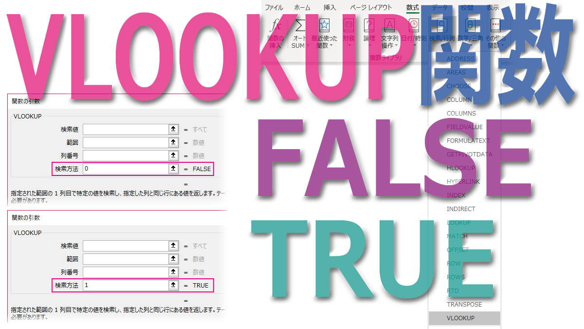
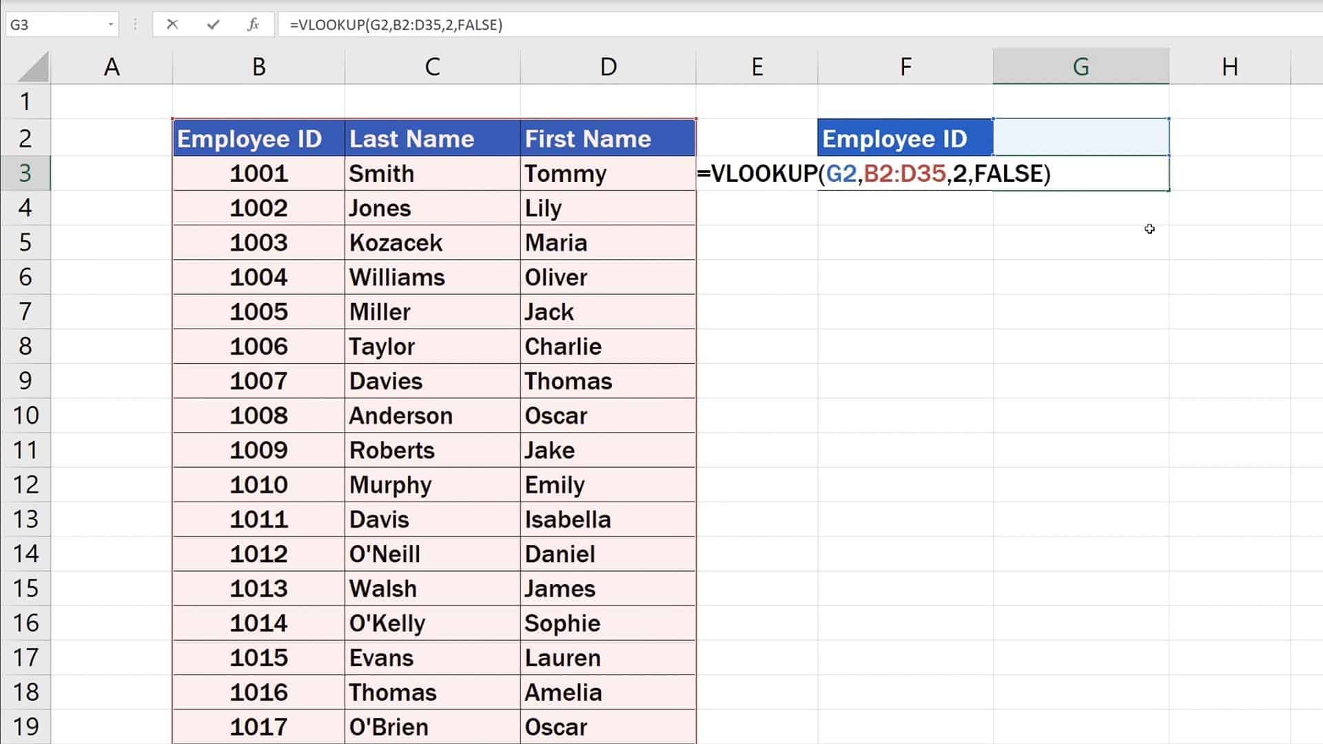
VLOOKUP (lookup_value, table_array, col_index_num, [range_lookup]) table_array: The range of cells to search for the lookup value. col_index_num: The column number that contains the return value. range_lookup: TRUE = approximate match, FALSE = exact match. Notice that the last argument allows you to specify TRUE to look for an approximate match.

Perbedaan True dan False Pada Fungsi Vlookup di Excel Tutorial Excel Pemula YouTube
If you don't specify anything, the default value will always be TRUE or approximate match. Now put all of the above together as follows: =VLOOKUP (lookup value, range containing the lookup value, the column number in the range containing the return value, Approximate match (TRUE) or Exact match (FALSE)).
Vlookup function with 'false' YouTube
The column index number is the number of columns Excel must count over to find the matching value. The VLOOKUP function also has an optional fourth argument: range lookup. This can be either TRUE or FALSE. If the range lookup argument is FALSE, VLOOKUP will find only exact matches. If the range lookup argument is TRUE, or if a range lookup.
How to use the VLOOKUP function
When using the VLOOKUP function in Excel, you can have multiple lookup tables. You can use the IF function to check whether a condition is met, and return one lookup table if TRUE and another lookup table if FALSE. 1. Create two named ranges: Table1 and Table2. 2. Select cell E4 and enter the VLOOKUP function shown below.
如何在Excel 2007和2010中正确使用VLOOKUP和True和False值 TurboFuture爱游戏客服中心 爱游戏 入口
Follow the steps to use FALSE in Excel VLOOKUP. Open the VLOOKUP function in the F3 cell. Choose the Lookup Value as an E3 cell. Next, choose the VLOOKUP table array as the Table 1 range. Column Index Number as 2. The last argument is [Range Lookup]. Mention it as TRUE or 1 in the first attempt.
VLOOKUP関数で「FALSE」と「TRUE」をどう使い分けるか TschoolBANK 作~るバンク
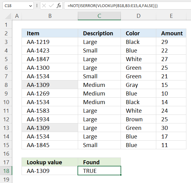
IF (VLOOKUP (…) = value, TRUE, FALSE) Translated in plain English, the formula instructs Excel to return True if Vlookup is true (i.e. equal to the specified value). If Vlookup is false (not equal to the specified value), the formula returns False. Below you will a find a few real-life uses of this IF Vlookup formula. Example 1.

Difference of true and false in vlookup, usage of true and false in vlookup, learn with Hany
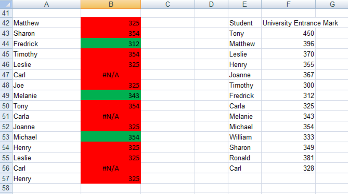
Excel Returns. TRUE. An exact, or approximate match. If Excel is unable to find an exact match, the next value that is less than the value you are interested in is returned. FALSE. An exact match. If Excel is unable to find a match, it returns #N/A. As you can see from the above table, Excel will return an approximate value if you choose TRUE.
如何在Excel 2007和2010中正确使用VLOOKUP和True和False值 TurboFuture爱游戏客服中心 爱游戏 入口
Vlookup is a crucial function for working with data in spreadsheets. Understanding true and false in vlookup is essential for accurate results. Using true in vlookup allows for an approximate match, while false requires an exact match. Common mistakes include mixing up true and false and not understanding the difference.
How to Use the VLOOKUP Function in Excel (Step by Step)
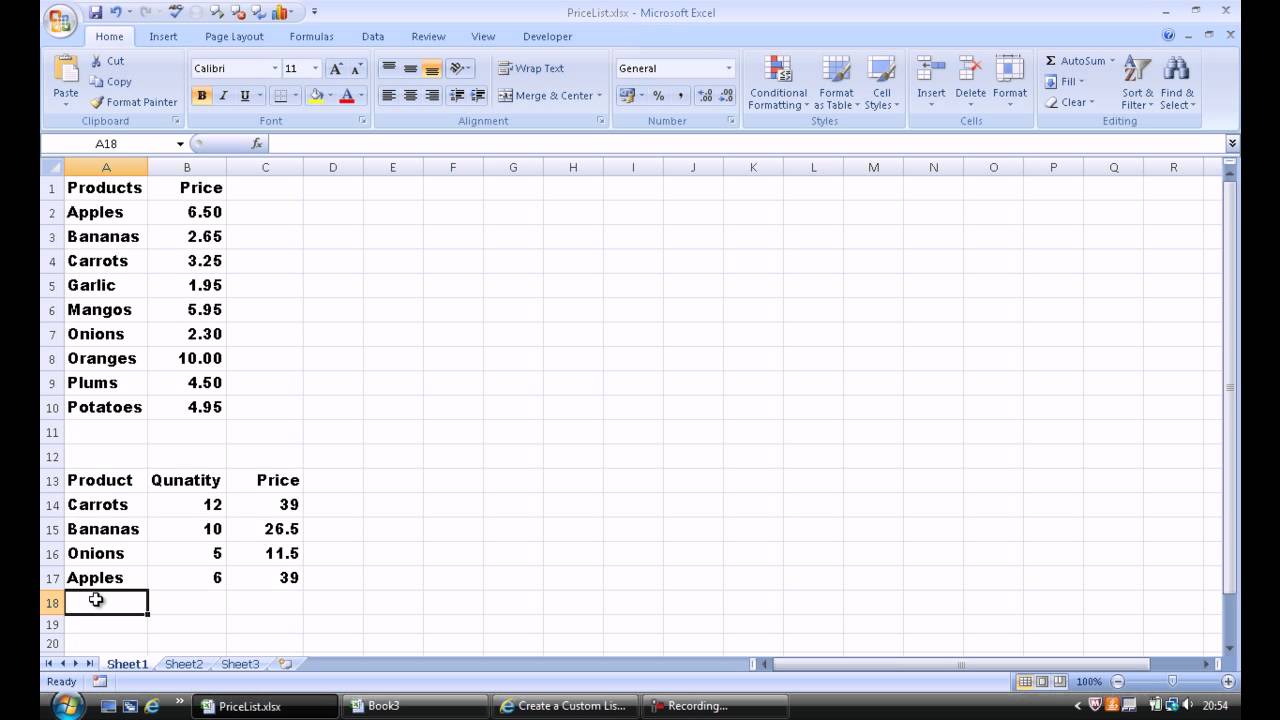
Short 2:18 video showing excel's Vlookup and when to use false for an exact match and true for a range. Chris Menard does Microsoft Office training in Atlan.

Perbedaan True dan False pada Rumus Vlookup di eXcel YouTube
FALSE = exact, TRUE = approximate (default). If range_lookup is omitted or TRUE: VLOOKUP will match the nearest value equal to or less than the lookup_value. Column 1 of table_array must be sorted in ascending order. If range_lookup is FALSE or zero for an exact match: VLOOKUP will perform an exact match. The table_array does not need to be sorted.
Excel Vlookup showing false and true arguments YouTube
Depending on whether you choose TRUE or FALSE, your formula may yield different results. Excel VLOOKUP exact match (FALSE) If range_lookup is set to FALSE, a Vlookup formula searches for a value that is exactly equal to the lookup value. If two or more matches are found, the 1st one is returned.

VLOOKUP ! TRICKS ! TRUE ! FALSE ! YouTube
VLOOKUP(E1, A5:B11, 2, FALSE) How to Vlookup and return multiple values in Excel. The Excel VLOOKUP function is designed to return just one match. Is there a way to Vlookup multiple instances? Yes, there is, though not an easy one. This requires a combined use of several functions such as INDEX, SMALL and ROW is an array formula.

Excel Vlookup False (lesson 1) YouTube
These two formulas are equivalent: = VLOOKUP ( value, data, column, FALSE) = VLOOKUP ( value, data, column, 0) In exact match mode, when VLOOKUP can't find a value, it will return #N/A. This a clear indication that the value isn't found in the table. 8. You can tell VLOOKUP to do an approximate match.
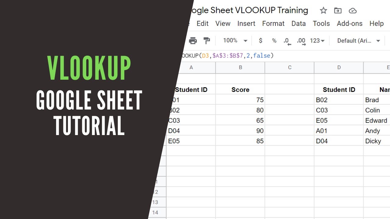
Google Sheet Tutorial VLOOKUP TRUE & FALSE Function YouTube
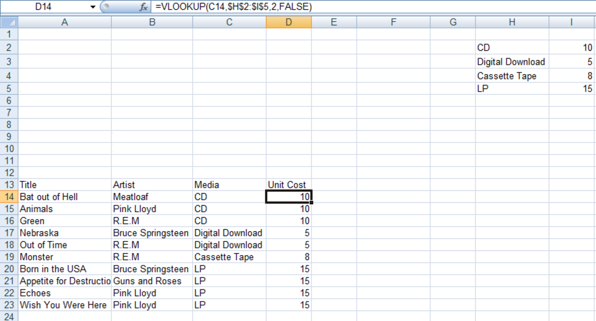
Here's an example of how to use VLOOKUP. =VLOOKUP(B2,C2:E7,3,TRUE) In this example,. Enter either TRUE or FALSE. If you enter TRUE, or leave the argument blank, the function returns an approximate match of the value you specify in the first argument. If you enter FALSE, the function will match the value provide by the first argument.

VLOOKUP Function Is Sorted (TRUE/FALSE) Google Sheets Formulas 8 YouTube
Returns. The VLOOKUP function returns any datatype such as a string, numeric, date, etc. If you specify FALSE for the approximate_match parameter and no exact match is found, then the VLOOKUP function will return #N/A. If you specify TRUE for the approximate_match parameter and no exact match is found, then the next smaller value is returned. If index_number is less than 1, the VLOOKUP.
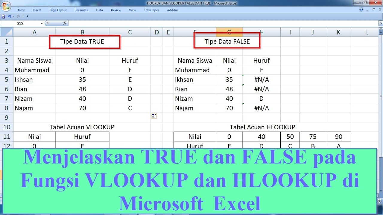
Menjelaskan TRUE dan FALSE pada Fungsi VLOOKUP dan HLOOKUP di Microsoft Excel YouTube
'FALSE' tells the VLOOKUP function to find an exact match, 'TRUE' tells the VLOOKUP function to find the nearest value that is still less than the lookup_value. Where the value is omitted the function will default to 'TRUE'. Until you understand how to use this correctly, it is best to use FALSE. In our example, our formula would be.
